Differences between Arbitrage betting and Dutching
Let’s pay closer attention to the below quantitative graph toward the difference between its main parts, Dutching area and Dutch books created in bookmaker favors
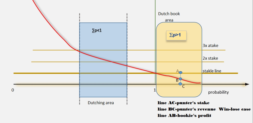
The very first thing that comes into the eyes have reflected in the main properties: ∑p>1 and ∑p<1which are in close relation with the profit (red) curve
In the area where is ∑p>1, values of the profit curve are under stake(line), while in the opposite case profit values are above the stake line
For ∑p=1 red curve crosses the stake line and that is the break-even case, no loss and no win case
Dutch book from another angle
For a reader who is for the first time visits this site I’ll provide a quick explanation on a real example for the left part, the Dutch book:
01 Oct 2022
1 X 2
Arsenal – Tottenham 2.07 3.62 3.41
p(1)=1/2.07=0.483092
p(0)=1/3.62=0.276243
p(2)=1/3.41=0.293255
∑p= 1.05259 > 1 => Dutch book on bookie’s side
Compound odds
What is the value in percent of the length of line BC?
Let’s do, this time, elementary math (for a complex approach see here)
The value of the stake line is S-our total stake
smaller parts, for covers, all basis (outcomes!) are respectively: s1,s0, and s2
In concrete case
s1+s0+s2=S ………………… I
We know that for a Dutch book must be fulfilled:
nrev=d1s1=d0s0=d2*s2 ………………………..II
If we put II in I then it follows:
nrev=S/(1/d1 +1/d0+1/d2) …………………III
The above formula allows us to introduce so-called compound odds, c.o:
nrev=S*c.o(d.0(1),d.o(0),d.o(2)
c.o(d.0(1),d.o(0),d.o(2)= 1/(1/d1 +1/d0+1/d2)
c.o=1/3*H(d.0(H),d.o(D),d.o(A)
function c.o, compound odds allows us to directly determine the revenue from the initial, undivided stake, S!
In concrete case, Harmonic mean(2.07,3.62,3.41)=2.85011
So compound odds have value:
c.o(2.07,3.62,3.41)= 0.950038
It means that the length of line BC is 95.0038% length of line CA
So, if we cover all outcomes, because Dutch book we will win one bet, but at the end we will return only 0.95 initial stake
We will be 0.05% on lose
The win-lose case is immanent for Dutch book from the punter’s perspective
Intro Dutching
Suppose we cover not all 3 but only 2 outcomes from considered example, say home win and draw
p(1)=1/2.07=0.483092
p(0)=1/3.62=0.276243
∑p= =0.75933 <1
In the same manner, it could be introduced formula for compound odds in this case:
c.o=1/2*H(d.0(H), d.O(D)=1.31649
If we deal with the unit stake then comes out
nrev=1*c.o=1.31649=1 + 0.31649*1=S+31.65%S
So profit is 31.65% from in 2 outcomes invested stake!
Not bad, but with one caveat-profit is not 100% sure!
Namely, there is a probability close to p(2)=29.326% to lose the bet!
Could we proceed with maximization in Dutching?
Why not, the process is the same as in Arb
All that is needed is to find and chose max odds from market different bookmakers!
In this particular case, for now, the max values are:
p(1)=2.12
p(0)=3.92
c.omax=1/2 H(2.12,3.92)= 1.37589404
Short historical sketches important for Dutching
Today’s punters have to give credit for this betting method to two prominent guys who originate not from scientific, but Jewish gangsters community
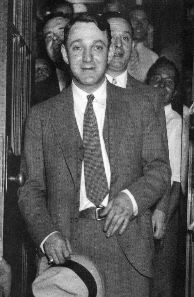
With his accountant, he invented principles for a method that is an object of our interest
His lucrative method requires a calculation machine which didn’t exist in the first third of the 20th century
Applying their method, Schultz bet at the track at the last minute in order to manipulate the odds and control what numbers came up so that no matter which one of them won, Shultz get the same payout.
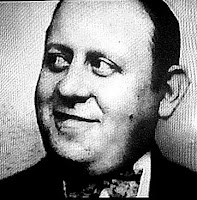
Schultz overcame that pure technical problem over his accountant and friend, Oto Bergman aka Abbadabba who was a math wiz being able mentally to calculate complex math operations in a second!
Among other things, Otto stays remembered because he coined the phrase: “Nothing personal, it is just business.“
Principles behinds Dutching
Let’s spice up our current consideration with a little bit of math with the very important term in Probability-random variables
Let X denote a (discrete!) variable from a bigger sample space with outcomes x1,x2,..,xn
X={ x1,x2,..,xn }
e.g. values x1,x2,..,xn can be the position of certain horses in a race on which one place bet
or in the same racing, an area where it primarily occurred Dutching means backing multiple horses to win in the same race
Form:

We have already often encountered random variables, but it wasn’t explicitly emphasized:
X=[H,D,A}
Variable X is a random variable because X=xp goes with probability, e.g. X=H(X will take value: H) goes with probability close to 1/d.o(H)
The same form of random variable X could be spanned on e.g. final score in football:
0-0, 1-1, 0-1 , 2-0….etc
or everything else you want to dutching on
Dutching Formula-derivation
Definition of necessary terms!
(To be honest, this step is not necessary, but I do it like a man who wants to give the impression that he knows what he’s doing 🙂
- allocation, α: coefficient for determent amount of particular stake in multiple lays
- dimension, δ: number of stakes
- combined odd, c.o : H(x1.x2,…xδ) /δ where:
- xi-particular decimal odd
- H-harmonic mean
- Potential, S : Total investment
- pi=1/xi : implied probability
Dutching core:
”Adjusting multiple stakes in a manner that you win equal revenue if either your selection win”
From above definition we stumble on :
- Flagenheimer-Bergman’s condition: “Adjusting multiple stakes…”
α1*S + α2*S +…. +αδ *S =S ð α1 + α2 +…. +αδ =1
From above we got:
Geometric interpretation of 1.F-B condition is delta dimensional polyhedral, Flagenheimer-Berghman’s polyhedral, F-B polyhedral
2. Flegenheimer-Bergman’s condition:
”…. win equal net income if either your selection win”
From here we got this:

Fundamental theorem of Dutching
If the 2nd F-B conditions are placed on the F-B polyhedron, then from the position of Potential (total stake!) exists multiplier, compound odds, which raises or lowers the actual potential
e.g. nrev=S*c.o(odds1,odds2,…,oddsδ)
proof:
α1 + α2 +…. +αδ =1 /*S
By multiplying like this, we get:
α1*S + α2*S +…. +αδ *S =S
Partial stakes:
α1*S=s(1)-partial stake on 1. outcome
α2*S=s(2)-partial stake on 2. outcome
etc.
That’s how we get:
s(1)+s(2)+….s(δ)=S ….I
from 2. F-B respectively is obtained:
s(1)=nrev/x1
s(2)=nrev/x2
.
.
etc up to δ
If we above put in I then follow:
nrev(1/x1 +1/x2 +….+1/xδ)=S
nrev=S/(1/x1 +1/x2 +….+1/xδ)) ……II
From here directly follows:
c.o(x1,x1,….,xδ)=1/δ *H(x1,x1,….,xδ) … III
Q.E.D
An example of real-world Dutching
Let’s have closer look at the next market:
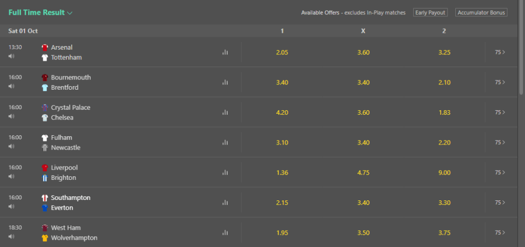
Say if our interest is half-time/Full-time outcome for Southampton-Everton:

In this type of market one encountering 3*3=9 options
To cover all options isn’t an option at all, because, you guessing-Dutch book
Let’s check:
∑p=1/3.6 +1/5.5+1/25+1/15+1/5.5+1/1/15+1/34+1/7.5+1/5.5
∑p =1.15931075
Compound odds,c.o:
c.o=1/∑p
c.o=0.86258149 => win-lose case
With arbitrage betting, Arb, we can win a bet but this win will result with 13.74% decreasing our initial stake, S !
Dutching in nothing else but reduction options played in Arb, so we must bounce out some ‘unnecessary’ options
How?
Which ones?
Here comes on its on the power of statistics.
Southampton as the home team is delegated by the bookmaker, odds 2.15
For applying dutching I filtered from the main statistic table all games from Premier Ligue where the home team delegated the next odds:
2.10, 2.14,2.15, 2.20 through a period of 15 years
Result:
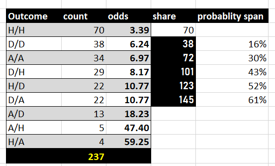
I decided to create the next random variable:
Xdutching={D/D, A/A,D/H,H/D,D/A}
The probability that variable X appear is 61% which is an excellent opportunity(in premium content I’ll explain why so and how to utilize it)
Compound odds for variable X:
c.o(X)=1/5*H(d.o(D/D),d.o(A/A),d.o(D/H),d.o(H/D),d.o(D/A))
c.o(X)= 1.341463
So with a (statistical!)probability of 61%, we can expect a 34.14% increasing initial bankroll, S
The story about Dutching isn’t exhausted because still stay find members(so-called: allocations) of F-B hipper plane:
α1 + α2 +α3 + α4 + α5 =1
and over them value partial stakes: s(1),s(2),s(3),s(4),s(5)
In the next post, I’ll cover this topic in a general case, mathematically precisely and comprehensively